Long-Term Monitoring Products

The long-term monitoring need

Natural resource managers are not only concerned with mapping and tracking disturbance events as they unfold in near-real-time. At longer time scales and often broader spatial scales, the need of planners and managers is to have inventories and assessments of slow-acting changes that are usually hard to map, quantify and interpret. While these slow-acting changes are easy to overlook, they can have profound influence on outcomes. This change includes incremental land use conversion, succession associated with altered disturbance or climate regimes, or gradual mortality or decline from invasive species.

Figure 1: Over the course of about five years, this Southern Appalachian riparian forest gradually lost nearly all of its Eastern and Carolina Hemlock to the progressive impacts of the non-native invasive Hemlock Woolly Adelgid. To address impacts, managers need to know where decline has occurred and the successional response of stands in subsequent years—both of these involve long-term monitoring. Photo credit: Steve Norman, USDA Forest Service.

Viewing ForWarn’s NDVI history provides a useful way to contextualize the impacts of one or more disturbances on the NDVI of a given pixel in ways that are not always evident or understandable from ForWarn’s near-real-time change maps. Near-real-time change products exploit ForWarn’s historical MODIS NDVI dataset by deriving different baselines for a specified period of the year. In contrast, long-term monitoring and analysis emphasizes inter-seasonal to inter-annual change, multiyear behavior such as attrition or recovery, and provides quantitative insights that can be used for predictive purposes.

Your ability to efficiently track short and long-term impacts is possible because ForWarn uses a continuous monitoring approach for the entire conterminous United States. Vegetation is systematically tracked, regardless of whether it has been disturbed or stressed or not. This provides rich monitoring insights about “normal” behavior, the cumulative effects of multiple disturbances, and the post-disturbance behavior that could be either recovery as expected or a vegetational type conversion.

Figure 2: The NDVI time series for this Southern Appalachian Eastern Hemlock forest in Great Smoky Mountains National Park shows how seasonal greenness changed over the course of 14 years. Beginning in the winter of 2006-7, winter NDVI plummeted, but it leveled off at a much lower state by the winter of 2010-11. By that time, the evergreen hemlock in this stand had succumbed to the Hemlock Woolly Adelgid. Also note the reduced decline in summer NDVI that reveals hemlock’s reduced contribution to the summer canopy. The ephemeral drop in early 2010 was caused by an unusually persistent snowpack that masked evergreen foliage across the region.

Figure 3: Contextual monitoring reveals change that would be easily overlooked by viewing change in terms of a short-term prior-year baseline. Areas with frequent disturbances, such as the repeat fires here in the Okefenokee National Wildlife Refuge, GA show the cumulative effects or gradual erosion of NDVI over time. Historically, fires were rare here, but they have become more frequent and severe through lower managed water levels and drought. (April 30, 2012, All Year Maximum Baseline).

Measures for long-term monitoring

The long-term condition of vegetation can be tracked by trends in the drivers of change through weather data, fire or insect occurrence databases, and also by the condition of the vegetation directly. The latter approach is also the monitoring approach used by the plot sample-based Forest Inventory and Analysis program (http://www.fia.fs.fed.us). In that ForWarn helps both recognize disturbances and track impacts, it provides a particularly useful toolset for integrative monitoring across programmatic efforts.

ForWarn’s historical database includes 46 NDVI products every year—a richness that results from having satellite overpasses each day and the ability to filter out clouds and poor atmospheric conditions. This temporal richness translates to phenological insights, such as the ability to recognize within-season changes from ephemeral disturbances and climate stress that would be otherwise undetectable or ambiguous, given the complexity of drivers at work in a given landscape. While no single phenological measure may be applicable across all vegetation types or geographic regions, numerous measures have been formulated that capture change that helps identify the causal drivers and the impacts that result. These include basic statistical measures, seasonal parameters, and annual percentiles as described below.

Basic annual measures

Useful monitoring insights can come from basic statistical measures such as each year’s median, maximum or minimum NDVI, and within-year variance or range. Similarly, the area under the annual NDVI curve (i.e., what ForWarn refers to as the large integral) tells us something about the type of vegetation present, annual productivity or the duration of the growing season. It is important to remember that these values are robust statistics, as they are generalized from 46 values for each year rather than derived from a single summer image, as often happens with Landsat, that may not be representative of the growing season or sensitive to change that occurs any time of year. Basic sub-annual (i.e., seasonal) values can also be calculated, such as the maximum value during the low-NDVI winter months—an alternative strategy to overcome false estimates of evergreen vegetation caused by heavy snowpack suppressing NDVI.

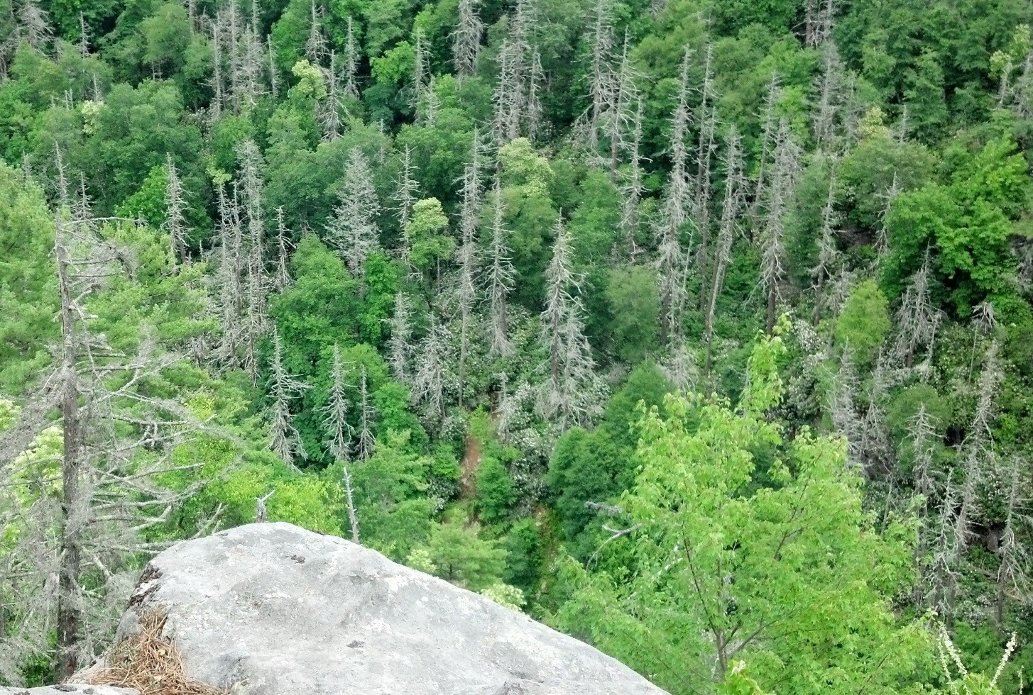
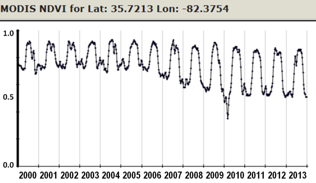
Interannual flux in these basic measures is caused by disturbance, successional recovery and often climate variation. Disturbance and recovery are manifest locally (Figure 4) while climatic variability that includes drought, snowpack depth or growing season productivity, is more generally landscape to regional in scope. As NDVI is an integrative measure for vegetation, its usefulness for specific measures of interest often needs to be demonstrated. For example, while it is well established that conifers are stressed by drought, their community response is less reliable than what is observed for grass-shrub or hardwood-mixed forest types.

Seasonal parameters and their derivatives

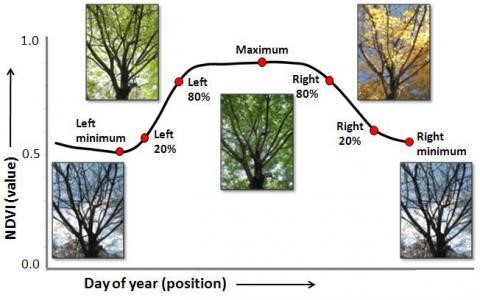
The classic land surface phenology curve for mid-latitude forests forms a hump with a rapid rise and fall that correspond to spring and autumn. While the basic form of this curve is dictated by seasonal factors governed by incoming solar radiation, variation in the year-to-year position of this curve usually reflects temperature or moisture conditions (Figure 5).

Seasonal parameters are intended to capture the date and NDVI values of these seasonal transitions and how they vary among years. By themselves, periodic NDVI values don’t tell us when the onset of spring or fall occurs, as values need to be kept in annual context. Severe disturbance can cause disruption in the normal NDVI progression such that decline occurs earlier than in undisturbed neighboring sites, even though the climate season per se has not changed. In general though, parameters mark biologically significant turning points in seasons such as when seasonal transitions occur. Those data provide a powerful measure for describing how climate affects vegetation responses.

ForWarn includes a suite of phenological products that characterize five seasonal transitions (Table below, Figure 6). Each year has two winter minimums, defined as “left minimum” and “right minimum”, and a single growing season “maximum”. Both the NDVI values and the day of year (or “position”) are determined. From these metrics, the 20th and 80th percent greenup values and dates for spring and the 80th and 20th percent values and dates for fall browndown are determined. With two maps for each of these seasonal parameters—the NDVI value and day of year position—there are 14 maps available for every year.

Figure 4: Seven seasonal parameters indicate transitions that include both NDVI values and the day of year. From these measures a number of derived measures are possible, such as the duration of the growing season and the rates of greenup and browndown.

Figure 5: Median greenup date based on the 20 Left parameter during 2000-2013 for all lands of the conterminous US. The median can be a more accurate measure of start of spring than the mean as the median reduces the false rise in NDVI that can occur with snowmelt that reveals understory evergreen vegetation. Spring generally commences 3-4 weeks later at higher than lower elevations or latitudes. Blue areas reflect these extremes or annual crop land use or desert climate conditions. In the desert Southwest, the 20 Left parameter does a relatively poor job capturing seasonal dynamics given phenological profiles that do not follow the phenological profile shown in Figure 4.

Two measures are associated with these seven seasonal parameters for each year–these are the NDVI value and the day of year when the parameter is achieved. This allows us to contrive measures based on changes in NDVI, changes in time or some combination of both, as in seasonal rates of change.

Annual percentiles

Percentiles of the annual distribution of NDVI values provide a different set of statistical tools for monitoring year to year change. The lower percentiles represent the non-growing season conditions and are often susceptible to persistent snowpack in colder climates. As discussed above, this snowpack can provide false lower values (percentiles with this approach) that obscure the evergreen fraction when deciduous vegetation is leafless in winter. The uppermost percentiles reflect conditions during the peak growing season. Where grass or shrubs comprise a portion of the observed vegetation, some periods of the year can be highly sensitive to seasonal weather conditions such as drought, and these are often manifest as variation in peak values or upper percentiles. This sensitivity of percentiles and the maximum to drought or snow can complicate interpretation of disturbance impacts. Use of percentiles allows monitors to tailor measures in ways that are more likely to approach the intended signal by eliminating extreme values that may be less trustworthy (Figure 6).

Figure 6: In the eastern US, the annual minimum is sensitive to winter evergreen cover, but also to variable snowpack. Capturing a somewhat higher percentile of the annual distribution better reflects variation in evergreen alone. For this map, regressed trends in the 25th percentile 2000-2011 reveal where winter evergreenness has declined as shown by dark grid cells. Most of the decline in Great Smoky Mountains National Park, southwest of it in the Joyce Kilmer Wilderness Area and east of Asheville result from gradual hemlock mortality from the Hemlock Woolly Adelgid. Other decline results from wildfires and harvesting in pine plantations, the latter of which is temporary. Maps such as this are useful for prioritizing landscapes for efficient monitoring and possible remediation.

Phenologically-based vegetation types

The NDVI profile of a grid cell can change considerably from one year to the next, but all change is not biologically important. Subtle differences in weather, ephemeral disturbance from minor storm events and atmospheric noise can distract from the vegetational information that is embedded in ForWarn’s NDVI time series. Moreover, with over 140 million MODIS pixels in the conterminous US, it is hard to make sense of so many different phenological profiles efficiently. Some type of classification or typing can be applied to make these data more useful and accessible.

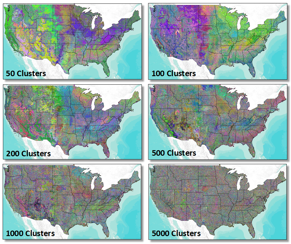
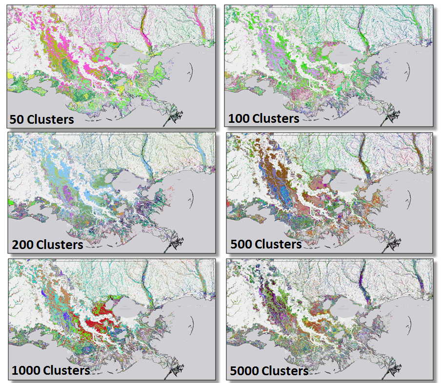
Statistical clustering of annual NDVI profiles provides a robust approach to classification. When just a few different clustered types are generated, the resultant types reveal only the most basic seasonal and productivity attributes. When a larger number of divisions are generated, subtle differences in productivity, the onset of spring or fall or nuances associated with disturbances can be resolved.

ForWarn uses non-hierarchical K-means clustering of the 46 NDVI values per year for all years in the dataset together, so that a single grid cell can potentially have membership in as many phenological categories as there are years of history. When relatively few clusters are generated, membership in a group is likely to be stable unless there is a severe disturbance. When several thousand types are generated, membership is more likely to shift. Clustering is performed with 50, 100, 200, 500, 1000 and 5000 divisions to provide different levels of division depending on classification needs (figure 7, 8).

Figure 7: Vegetation types based on phenologically similar NDVI profiles according to different levels of division. These maps show the “max-mode” grouping which is the most frequent grouping from 2000-2012; when there are ties or no mode, the maximum area under the curve is used. With low divisions, groupings strongly resemble traditional ecological regions. Random colors are used in these maps. At higher division, finer differences in phenological type can be discerned as shown in figure 8 below.

Figure 8: Phenologically-based groups for wetlands of the bottomlands of the Lower Mississippi based on the max mode for 2000-2012 and using random colors (see caption in Figure 7 for details).

These phenologically-based vegetation types are calculated annually so that shifts in membership from one type to the next can be tracked more efficiently than is possible when raw NDVI profiles are used. Membership shifts over time is useful for vegetational transition and successional modeling, prioritization efforts, and assessment of vegetation patterns and representation of biologically important changes over time.

Putting long-term monitoring to work

Any of the annual or seasonal derived products described above could be used for long-term forest or landscape monitoring. The measure selected should be closely aligned with the management question asked and the ability of that measure to function fairly for a particular ecosystem or climate.

Some of the most promising applications of long-term NDVI data are these:

• Efficient mapping of evergreen or deciduous decline
• Efficient mapping of evergreen or deciduous recovery
• Coarse prioritization of areas of concern within a landscape
• Successional dynamics of NDVI types
• Robust characterization of normal behavior for contextualizing change